Quickstart#

This notebook shows how to create a synthetic graph and then how to train a model in a classification task using Haiku Geometric.

Haiku Geometric - Graph Neural Networks in JAX#

Haiku Geometric is a collection of graph neural network (GNN) implementations in JAX. It tries to provide object-oriented and easy-to-use modules for GNNs.

Haiku Geometric is built on top of Haiku and Jraph. It is deeply inspired by PyTorch Geometric. In most cases, Haiku Geometric tries to replicate the API of PyTorch Geometric to allow code sharing between the two.

Haiku Geometric is still under development and I would advise against using it in production.

You can find all the available graph neural network layers here.
Visit also Haiku Geometric documentation.

Creating a synthetic graph#

We will create the following graph:

synthetic graph

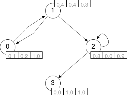
To do so, we create the following variables:

nodes: a 2D array of shape [num_nodes, num_node_features] with features.
senders: a 1D array of shape [num_edges] with the source edge node indices.’
receivers: a 1D array of shape [num_edges] with the destination edge node indices.’

[1]:

import jax.numpy as jnp

nodes = jnp.array([
    [0.1, 0.2, 1.0], # node 0 features
    [0.4, 0.4, 0.3], # node 1 features
    [0.8, 0.0, 0.9], # node 2 features
    [0.0, 1.0, 1.0]  # node 3 features
])
senders = jnp.array([0, 1, 1, 2, 2])
receivers = jnp.array([1, 0, 2, 2, 3])

WARNING:jax._src.lib.xla_bridge:No GPU/TPU found, falling back to CPU. (Set TF_CPP_MIN_LOG_LEVEL=0 and rerun for more info.)

Creating a model#

We will create a model with 2 graph convolutional networks (haiku-geometric.nn.GCNConv) layers followed by a linear (hk.Linear) layer. Notice that to do so we group our layer in a new Haiku module denoted MyNet.

[2]:

import jax
import haiku as hk
from haiku_geometric.nn import GCNConv

class MyNet(hk.Module):
    def __init__(self, hidden_channels, out_channels):
        super().__init__()
        self.conv1 = GCNConv(hidden_channels)
        self.conv2 = GCNConv(hidden_channels)
        self.linear = hk.Linear(out_channels)

    def __call__(self, nodes,senders, receivers):
        x = self.conv1(nodes, senders, receivers)
        x = jax.nn.relu(x)
        x = self.conv2(x, senders, receivers)
        x = self.linear(nodes)
        return x

Transforming the model#

We now define a forward function that instantiates the net and performs a call. This function will be transformed by Haiku and will perform a forward pass on the model.

[3]:

def forward(nodes, senders, receivers):
    net = MyNet(16, 7)
    return net(nodes, senders, receivers)

Finally, we transform the forward function as explained in the Haiku documentation. After transforming the function, we have to initialize the model with the init function that receives our graph data.

[4]:

model = hk.transform(forward)
model = hk.without_apply_rng(model)
rng = jax.random.PRNGKey(42)
params = model.init(rng, nodes=nodes, senders=senders, receivers=receivers)

After this, we are ready to perform a forward pass on the model.

[5]:

output = model.apply(params, nodes=nodes, senders=senders, receivers=receivers)
output

[5]:

DeviceArray([[ 0.00770418, -0.7566054 ,  0.51024306,  0.2543769 ,
               0.4244291 ,  1.0645634 , -0.30671927],
             [-0.10649211, -0.5037036 ,  0.24744353,  0.20532413,
               0.06193589,  0.6883482 ,  0.1389835 ],
             [ 0.27398756, -0.32722455,  0.59584326, -0.2710259 ,
               0.59495777,  1.479022  ,  0.37957942],
             [-0.47271663, -1.6297377 ,  0.53237855,  1.0204307 ,
               0.07947233,  1.1653316 , -0.5966778 ]], dtype=float32)

Learning on graphs#

Lets say that we want to perform classification on the graph. We will consider the following array of ground truth labels (one class for each node) that we will try to predict:

[6]:

labels = jnp.array([0, 1, 2, 0])

We are ready to perform learning with our model (e.g. with gradient descent). To do so we will use an optimizer from optax. In this case we will use the Adam optimizer.

[ ]:

!pip install optax

[7]:

import optax

opt_init, opt_update = optax.adam(learning_rate=0.1)
opt_state = opt_init(params)

We define out loss function, where we first performa a forward pass to computed the logits, ant the compute the loss, in this case, softmax cross entropy loss. Notice that the function is JAX compatible and we can use the jax.jit decorator to speed up the training.

[8]:

@jax.jit
def loss_fn(params):
    logits = model.apply(params, nodes=nodes, senders=senders, receivers=receivers)
    x_loss = optax.softmax_cross_entropy_with_integer_labels(logits, labels)
    return jnp.sum(x_loss)

We also define a function that computes the gradients of the loss function ( by using the jax.grad function) and updates the model parameters.

[9]:

@jax.jit
def update(params, opt_state):
    g = jax.grad(loss_fn)(params)
    updates, opt_state = opt_update(g, opt_state)
    return optax.apply_updates(params, updates), opt_state

We will also need a function that computes the accuracy of the model. Again, this function is compatible with the jax.jit decorator.

[10]:

@jax.jit
def accuracy(params):
    logits = model.apply(params, nodes=nodes, senders=senders, receivers=receivers)
    return jnp.mean(jnp.argmax(logits, axis=-1) == labels)

Finally, we can perform the training loop! We will train for 10 epochs:

[11]:

for step in range(10):
    params, opt_state = update(params, opt_state)
    acc = accuracy(params)
    print(f"Step {step}: accuracy = {acc}")

Step 0: accuracy = 0.0
Step 1: accuracy = 0.25
Step 2: accuracy = 0.25
Step 3: accuracy = 0.25
Step 4: accuracy = 0.5
Step 5: accuracy = 0.75
Step 6: accuracy = 1.0
Step 7: accuracy = 1.0
Step 8: accuracy = 1.0
Step 9: accuracy = 1.0

Haiku Geometric

Quickstart

Contents